Measuring combat effectiveness: a novel method based on two-dimensional frontline advancement rate

Accurately measuring combat effectiveness is a cornerstone of military and political science research. Lanchester (1916) laid the foundation for this field with his renowned Lanchester equations, which focus on quantifying casualties based on the number of engaged combatants. These equations have profoundly influenced subsequent research, inspiring numerous variants over the decades. Notable adaptations include Dolanský’s (1964) and Novikov’s (2013) formulations, with Helmbold’s (1997) variant standing out for its significant contributions. Furthermore, comprehensive compilations by Przemieniecki (2000) and Tolk (2012) have incorporated a wide range of advanced combat models derived from these equations. However, despite these refinements, these variants remain rooted in Lanchester’s original framework, relying on the number of combatants as the primary measure of combat effectiveness. The mathematical sophistication introduced by these studies enriches the modeling but does not fundamentally deviate from Lanchester’s foundational approach.

In contrast, researchers such as Hayward (1968) sought to expand the scope of explanatory variables beyond the number of participants. Hayward proposed a mathematical model that incorporates three primary dimensions: (a) capabilities, (b) environment, and (c) missions. This innovative framework was subsequently adopted and further developed by scholars including Epstein (1985), Dupuy(1987), Krondak et al. (2007), Talmadge (2013), Kanatliev (2014), and Gordon (2014).

The common feature of the aforementioned approaches lies in their reliance on attributes (explanatory variables) as the basis for measurement. They aim to establish a mathematical model—one that, given the known attributes, could calculate combat effectiveness. However, this measurement approach suffers from two inherent flaws:

Firstly, the complex synergy of numerous contributing factors determines combat effectiveness, making it impossible to elaborate on every detail. For instance, there is a strong correlation between scientific and technological development and increased combat effectiveness. However, the term “level of S&T development” is overly broad; even professional S&T reviewers struggle to account for every scientific and technological achievement and its military application. In addition to S&T development, combat effectiveness relies on a multitude of equally encompassing factors that may vary in their intercorrelations, including organizational, individual, tactical, strategic, and environmental factors. Indeed, Hayward acknowledges that “even the most thoroughgoing analysis will leave a rather large number of independent variables, the influence of which on combat effectiveness remains to be assessed” (Hayward 1968, p. 322).

Secondly, even if researchers could identify all the factors contributing to combat effectiveness, they would still encounter difficulties in quantifying perceptual and non-measurable elements. For instance, Epstein (1985) questioned the practical applicability of the Lanchester equations and proposed an alternative model incorporating additional combat parameters, such as the marginal utility of extra soldiers and public tolerance for military and civilian casualties. However, these parameters remain inherently unmeasurable and can only be hypothesized. As Nigel Perry (2009, p. 20) points out, the inability to quantify such parameters is a common limitation across existing combat models.

As the academic community gradually recognized the challenges of establishing precise combat models based on explanatory variables, contemporary political science research has shifted toward a two-step approach. Researchers now tend to first measure combat effectiveness using the Loss Exchange Ratio (LER) method and then employ statistical techniques to explore the relationships between various combat attributes (explanatory variables) and combat effectiveness based on the obtained data. Early works in this area include Millet et al. (1986) and Reiter and Stam (1998). Since the turn of the century, significant contributions have been made by Pollack (2002), Desch (2002/2008), Biddle and Long (2004), Farrell (2005), Brooks and Stanley (2007), Downes (2009), and Lyall and Wilson (2009). In the 2010s, influential studies were produced by Millett and Murray (2010), Beckley (2010), Biddle (2010), Friedman (2011), Pilster and Böhmelt (2011), Johnson (2012), Apostolou (2015), and Reiter (2017). More recently, ongoing discussions have continued to shape the field, with notable works by Reiter (2020, 2022), Lyall (2020), Grauer and Quackenbush (2021), Plapinger (2022), Kuo (2022), and Mehrl (2022).

The prominence and favorability of the LER method among researchers stem from its reliance on outcome variables rather than explanatory variables for measurement. This approach significantly reduces measurement complexity while improving accuracy. Although the LER method may seem similar to Lanchester’s equations, as both use the number of soldiers as a basis for measurement—replacing the number of combatants with the number of casualties—there is a fundamental distinction between the two. In Lanchester’s equations, the number of participants serves as the cause of combat effectiveness, or the explanatory variable, whereas in the LER method, the number of casualties represents the effect, or the outcome variable.

By using outcome variables as a basis for measurement, the LER method addresses two major issues associated with relying on explanatory variables: the proliferation of explanatory variables and the inclusion of many immeasurable subjective factors. Measurement based on explanatory variables requires a comprehensive enumeration of all relevant factors, as omitting any variable could result in an incomplete representation of combat effectiveness. In contrast, when measuring from the perspective of outcome variables, only the most effective and objective results need to be considered, even if a variable may yield multiple outcomes.

Consider temperature measurement as an example. For temperature, factors such as solar radiation, geothermal energy, atmospheric conditions, human activity, and various natural or artificial chemical reactions serve as causes, or explanatory variables, or independent variables. This is analogous to the relationship between “the number of combatants” and “combat effectiveness.” To measure temperature using these explanatory variables, they must be integrated into a comprehensive mathematical model without omission. Missing any of these variables could result in an incomplete assessment of temperature. However, exhaustively accounting for all these diverse variables is nearly impossible, particularly given the inherently unquantifiable subjectivity of factors related to human activity.

In contrast, factors like phase changes in water or alcohol, as well as varying human perceptions of cold and heat, serve as effects, or outcome variables, or dependent variables. This parallels the relationship between “casualty numbers” and “combat effectiveness.” There is no need to unify all these outcomes into a single model; rather, it suffices to select the most universal and objective measure among them—the phase transition of water—as the basis for measurement. Indeed, this principle underlies the establishment of the Celsius and Fahrenheit temperature scales.

The next question is whether personnel casualties are the most appropriate outcome variable for measuring combat effectiveness. I believe there are two significant areas for improvement:

First, obtaining accurate figures for personnel casualties from battle reports remains a daunting challenge. These reports are often influenced by motives to overstate enemy casualties while downplaying one’s own, aiming to boost morale, undermine the enemy’s confidence, and garner the trust of allies. Even data on war losses published long after the conflict ends are similarly affected by the desire to conceal one’s own casualties while exaggerating those of the enemy, which serves to enhance historical evaluations and bolster national pride. Furthermore, official figures often originate from the reports of front-line commanders, who may have incentives to minimize their own losses and inflate enemy casualties to improve their promotion prospects (Obermeyer et al. 2008). While current solutions involve more rigorous scrutiny of data sources without altering the measurement methodology, such as recent LER collections that employ triangulation with multiple secondary historical sources and adjustments made by professional historians interpreting primary data, this approach still operates within the framework of personnel casualties.

Second, according to a widely accepted definition (McKenna, n.d.), combat effectiveness is defined as the ability to win battles. Thus, the most direct outcomes for measuring combat effectiveness are victory, draw, and defeat. By essentially measuring kill effectiveness—one means of achieving victory—LER only provides an indirect measure of combat effectiveness, which does not align with these direct outcomes. Historically, there are numerous examples where forces displayed valor and achieved disproportionate kill ratios (e.g., during the Winter War, Finland’s LER was 4.898), yet ultimately suffered defeat, as well as instances where victories were secured at significant cost (e.g., during the Winter War, the Soviet Union’s LER was 0.204).[1]

Therefore, the purpose of this paper is to identify a variable for measuring combat effectiveness that is more suitable than LER. This variable should meet the following three criteria:

1.It is an outcome variable of combat effectiveness.

2.There is no subjective interference in the acquisition of data.

3.It is a quantitative variable, which consistently aligns with the categorical variables of victory, draw, and defeat.

Method

We believe that frontline changes serve as a more suitable variable for measuring combat effectiveness for the following reasons:

1.Frontline changes are an outcome variable of combat effectiveness, as combat effectiveness drives changes in the frontline, not the other way around.

2.Frontline changes offer technical guarantees regarding the objectivity of data collection. In previous conflicts, photographs taken by embedded journalists and the abundance of relics left at battle sites make changes in the frontline more public and verifiable compared to casualty figures. More importantly, the advent of modern satellite technology, which can capture imagery of war zones from space and utilize short-wave infrared (SWIR) devices to monitor the operational positions of thermal weapons, significantly reduces the potential for falsification in frontline position data. Modern satellite technology allows for the collection of high-resolution imagery, providing unparalleled views of conflict zones. This capability ensures that movements and changes in frontlines can be monitored accurately, offering real-time data critical for strategic decision-making. Furthermore, these satellites can circumvent traditional limitations such as geographical barriers and access issues, providing a comprehensive overview of the battlefield. SWIR devices can detect heat signatures from various military assets, including vehicles and weaponry, even under limited visibility conditions such as smoke, fog, or darkness. When both parties engage in combat using modern thermal weapons along the frontline, the engagement positions can be quickly and accurately captured by SWIR devices.

3.Clausewitz (1976, p. 90) asserts that the ultimate goal of war is to subjugate the adversary’s territory under one’s authority, indicating that the essence of war is a struggle for control over power. This aligns with traditional military interpretations: when Party A successfully extends its control into Party B’s territory, it signifies that Party A’s frontline advances while Party B’s recedes, reflecting a victory for Party A and a defeat for Party B. Conversely, when neither party can assert control within the other’s territory, resulting in an unchanged frontline, this scenario is typically recognized as a draw.

The next challenge lies in quantifying changes in the frontline. Previous researchers have commonly used the distance or speed of army advancement within enemy territory as a measure. Helmbold (1990) reviewed studies from the Cold War period that employed this approach. Research in this area has continued beyond 1991; for instance, Biddle (2006/2010) and Grauer (2016) utilized advancement speed as a metric for territorial gains. Han (2016) further developed software capable of predicting marching speed based on input explanatory variables of combat effectiveness. However, this method of quantification suffers from at least two key limitations:

Reason I:

The intricacy of military engagements means that the trajectory of an army advancing within enemy territory is complex and variable, rather than a straightforward or constant forward movement. Consider two armies, A and B. Army A spends considerable time capturing four regions—P, Q, R, and S—progressing from the border into enemy territory. Each region is methodically and securely occupied, reflecting a slow but steady advance. In contrast, after breaking through the enemy’s front, Army B, unable to establish a stable foothold, captures P only to abandon it in order to take Q, then relinquishes Q to seize R, and finally abandons R to occupy S. Although Army A is demonstrably more effective in altering the frontline, its total marching distance is equal to that of Army B, and its speed may appear slower in comparison

Reason II:

Advancement speed fails to account for the multidimensional nature of the frontline. Profoundly penetrating enemy territory alters only one dimension of the frontline—the vertical depth—while neglecting another crucial dimension: the width of the front. For instance, if Army A achieves a breakthrough on a narrow front, just a few hundred meters or kilometers wide, it resembles a needle piercing the enemy’s frontline. In contrast, Army B breaches the enemy’s frontline at the same advancing speed but across a broad front spanning tens or even hundreds of kilometers, akin to a wave crashing onto the shoreline at high tide. The degree of disruption inflicted on the enemy’s frontline by Army A is significantly less than that caused by Army B, despite both armies having identical marching distances and speeds.

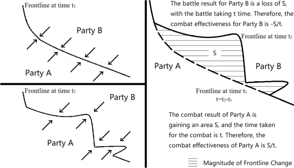
To address the aforementioned two issues, the one-dimensional linear advancement speed should be replaced with a two-dimensional planar advancement speed, which incorporates two key elements: the area (S) enclosed by the new and old frontlines, and the time (t) taken for the frontline to shift from the old to the new position.

Consequently, we propose the following formula to measure combat effectiveness:

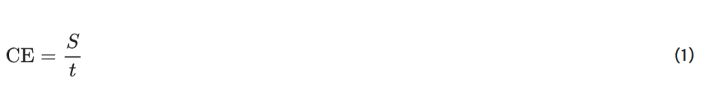
Area is measured in square meters (sqm) or square kilometers (sqkm), while time is measured in hours (h) or years (a). Therefore, the basic unit for measuring combat effectiveness is square meters per hour (sqm/h) or square kilometers per year (sqkm/a). We designate this new approach to measuring combat effectiveness as the TFR (Two-Dimensional Frontline Advancement Rate) method, as illustrated in Fig.1

An important point to note is that frontline changes should not be conflated with territorial changes. For example, in the Battle of Friedland in 1807, Napoleon defeated the Russian Imperial Army on Prussian territory, forcing them to retreat to the Russian border (Niemen River). The speed of the changes in the frontlines reflected the superior combat effectiveness of the French army over that of the Russian Empire. However, the territorial boundaries of the Russian Empire were not altered as a result of this battle. In fact, following the Treaty of Tilsit signed after this battle, Russia actually expanded by acquiring part of Prussia’s territory, as Napoleon sought to entice Tsar Alexander I into an alliance. This illustrates that our method focuses solely on the ability of armies to alter the frontlines on the battlefield due to the combined effects of various factors. Whether these changes in the frontlines result in territorial shifts is irrelevant to our method.

In most cases, territorial changes during a war between two nation—states correspond to shifts in the front lines, as exemplified by the ongoing Russo—Ukrainian conflict. Since 2014, the two sides have reached no diplomatic agreement on redrawing their borders, so any changes in territorial control have been solely the result of military confrontation. In contrast, once a war ends, the final territorial changes often diverge from the earlier front—line shifts because various non—military factors influence postwar border agreements. For example, historical records indicate that the British Empire expanded by about 25.9 Tsqm [2] during the nineteenth century (Levine 2013, p. 92). This figure does not match the actual territorial advances achieved on the battlefield and thus cannot be used to evaluate the overseas combat effectiveness of British forces.

The Opium Wars provide a typical illustration. During the military phases of both conflicts, British troops pushed the front lines to Nanjing (Chinese for “Southern Capital”) and Beijing (Chinese for “Northern Capital”), which corresponded to increases of approximately 28 Gsqm and 35 Gsqm, respectively. These figures can serve as a metric for assessing the overseas combat effectiveness of the British army. However, because Britain’s strategic objective was not to become China’s new ruler but rather to expand free—trade markets, the final outcome of these two wars involved relinquishing the occupation of these major Chinese political centers. Consequently, the only territorial changes were limited to two coastal trading outposts—Hong Kong Island and the southern tip of the Kowloon Peninsula—leading to incremental area gains of roughly 79 Maqm and 11 Msqm, respectively. Clearly, this outcome, which is one of the components of Levine’s (2013) statistical data on the overseas territorial expansion of the British Empire in the nineteenth century, is not suitable for measuring the overseas combat effectiveness of the British military.

Therefore, first, our method is not only applicable to conflicts between nations but also to conflicts between any entities, as long as clear frontlines exist between them. While territory is an exclusive concept of nation-states, frontlines are not. For example, civil wars and guerrilla warfare occur within a single country (with the key difference being whether the opposition is on par with the government forces) and do not result in changes to national territory. However, both create frontlines distinct from government-controlled areas, which evolve as battles progress.

Second, our method is not limited to wars motivated by territorial acquisition but also applies to conflicts driven by any other motivation, as long as such motivation leads to the delineation of clear frontlines. For instance, wars of revenge or wars aimed at maintaining international law and order may not be driven by territorial conquest, yet they still create distinct frontlines between opposing forces. A case in point is the war between the United States and Japan during World War II, which had a dual motive: revenge for the Pearl Harbor attack and the liberation of Asia–Pacific nations suffering from Japanese aggression. Thus, while the war did not ultimately change the territorial boundaries of the United States and Japan, each battle resulted in changes to the frontlines. This is because, although the United States had no territorial ambitions regarding Japan, achieving these two objectives still necessitated pushing the frontlines toward Japan.

Monadic CE and dyadic CE

Monadic Combat Effectiveness refers to the pure combat effectiveness possessed by a military force, evaluated independently of specific adversaries. The assessment primarily relies on intrinsic factors such as the size of the military, the advancement of its weaponry, the physical fitness of its personnel, and the level of military theory in use. For instance, a country with a large number of troops equipped with advanced weapons like fighter jets and tanks, along with well-trained soldiers, can be said to have high monadic combat effectiveness.

Dyadic Combat Effectiveness, in contrast, focuses on the level of combat effectiveness displayed by a military force in relation to its specific adversaries. For instance, a military might possess high monadic combat effectiveness, but when faced with an opponent with even greater monadic combat effectiveness, it could still suffer defeat, which reflects low dyadic combat effectiveness.

What our formula measures is dyadic combat effectiveness

Since dyadic combat effectiveness essentially represents the difference between two monadic combat effectiveness values, the combat effectiveness sign in the TFR method is expressed as CE_A−B, which is equivalent to CE_A − CE_B. Therefore, in our method, when “CE = 0” is measured (indicating that the frontlines remain static or that their positions are the same before and after the battle), it signifies that the monadic combat effectiveness of both sides is equal. This can be likened to two cars traveling in the same direction at high speed: while their absolute velocity is quite high relative to the ground or a fixed point, their relative velocity is zero if they travel at the same speed. Similarly, in a tug-of-war, if the rope remains stationary, it does not mean that both sides exert zero force; rather, it indicates that their forces are equal, resulting in no disparity in strength.

Example I

In the battles of Verdun and the Somme on the Western Front during World War I, despite the massive mobilization and heavy casualties sustained by both the French and British forces and the German army, the frontline did not undergo any significant change. According to our measurement formula, CE = 0. This initially seems puzzling; however, it becomes clearer when one recognizes that CE = 0 does not imply that the monadic combat effectiveness of the Entente and German forces was zero, but rather that their monadic combat effectiveness was equal.

Proof

There would have been no need for either side to engage in such prolonged and brutal battles for control over locations like Verdun and the Somme if one side had possessed a decisive advantage in combat effectiveness. Had the Entente forces held a clear advantage, they might have been expected to repel the German forces and potentially advance as far as Berlin, akin to the Soviet army’s advance during the later stages of World War II. Conversely, if the Germans had demonstrated superior combat effectiveness compared to the Entente, they would likely have succeeded in capturing Paris, as they had in the early phases of World War I. The inability of either side to achieve its strategic objectives underscores the absence of a clear advantage in combat effectiveness, ultimately leading to the protracted confrontations at Verdun and the Somme.

Example II

During the tug-of-war in the first year of the Korean War, both sides found that once they crossed the 38th parallel, defeating the opponent became implausible. Consequently, the front line stabilized near the 38th parallel in the summer of 1951 and remained there until the conclusion of the war. According to the measurement formula, CE_{PRC&DPRK—US&ROK} = 0.

Proof

Similar to the previous example of the Western Front during World War I from 1915 to 1916, if the US and South Korean forces had exhibited a higher level of combat effectiveness than their opponents, they would have advanced to the Yalu River. Conversely, if the Chinese and North Korean coalition had demonstrated superior combat effectiveness, they would have pushed forward to Pusan (Halberstam, 2007). In reality, neither of these scenarios transpired, indicating that neither side possessed a decisive advantage in combat effectiveness relative to the other.

Example III

In the ongoing Russo-Ukrainian War, a similar scenario of strategic stalemate has emerged, characterized by a “CE = 0”. In 2023, neither Russia’s early-year offensive on Bakhmut nor Ukraine’s summer counteroffensive produced any significant shift in the front line. This new battlefield deadlock has persisted for over a year, marking a distinct shift in the conflict’s dynamics. According to the measurement formula, CE_{Russia−Ukraine} = 0.

Proof

This follows a similar logic as in the previous examples: if Russia’s combat effectiveness were higher than Ukraine’s, it would have achieved its initial objectives of capturing Kyiv and potentially all of Ukraine. Conversely, if Ukraine’s combat effectiveness were superior, it would have successfully regained all lost territory. However, the inability of either side to achieve its strategic objectives indicates that their combat effectiveness levels are equal.

The proof process for the three specific cases above can be generalized to all similar cases using the following logical reasoning:

If the force P cannot achieve its strategic goals, it means that its combat effectiveness is not higher than Q (if not, P can compete and win with Q), i.e., CE_P ≤ CE_Q.

If the force Q cannot achieve its strategic goals, its combat effectiveness is not higher than P (if not, Q can compete and win with P), i.e., CE_Q ≤ CE_P.

The strategic stalemate means that neither party can achieve their respective strategic goals. In other words, it implies that the following two inequalities:

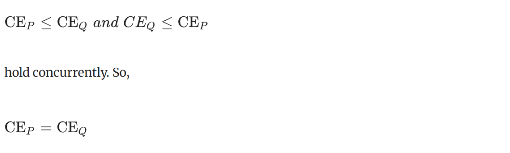
Thus, the “zero value” (situated between positive and negative values) in the TFR method effectively encapsulates the essential characteristics of a “strategic stalemate” or “draw,” as traditionally described in military discourse—positions that lie between victory and defeat.

Despite the logical proof presented above, the results may not be readily comprehensible to all readers. The situation of “CE = 0” on the Western Front during World War I—among the British, French, and Germans, all considered military powers—is relatively straightforward to understand. However, it is more challenging to grasp how the newly established People’s Republic of China (PRC) could achieve a “CE = 0” against the United States, the world’s most powerful nation following World War II. Similarly, it is difficult to comprehend how Ukraine, a country with a moderate international military ranking, could reach a “CE = 0” scenario with Russia, the pre-war second-ranked military power globally. The explanation for these two cases of “CE = 0” lies in another classification that will be discussed next: the distinction between theoretical combat effectiveness and tactical combat effectiveness.

Theoretical CE and tactical CE

Theoretical Combat Effectiveness refers to the combat effectiveness derived from the theoretical integration of various contributing factors that determine its value. It is a predictive assessment of potential combat effectiveness obtained through professional analytical methods, based on known information and data, prior to actual engagement in combat. For instance, a military force with a large number of highly trained soldiers, advanced weapon systems, robust logistical support, and effective command structures would be assessed to have high theoretical combat effectiveness.

Tactical Combat Effectiveness, in contrast, refers to the actual combat effectiveness value demonstrated by a military force in real combat situations. For example, a military unit may possess high theoretical combat effectiveness due to its superior training and equipment, but if the unit faces unexpected and theoretically easy-to-overlook contingencies on the battlefield—such as rare epidemics or sudden betrayal by allies—it may experience tactical combat effectiveness that is very low.

What our formula measures is tactical combat effectiveness

Murray and Millett (2010) classify military effectiveness into four levels: the political level (leadership by military leaders and formulation of military policies), the strategic level (comprehensive strategic planning), the operational level (detailed campaign planning), and the tactical level (direct combat actions executed by frontline units). Theoretical combat effectiveness is primarily associated with the first three levels, reflecting a nation’s capacity derived from political leadership, strategic foresight, and operational planning. In contrast, tactical combat effectiveness aligns with the tactical level, representing actual battlefield outcomes as the aggregate effect of various explanatory variables. The distinction between theoretical combat effectiveness and tactical combat effectiveness can be likened to the comparison between a car’s maximum design speed and its actual driving speed, or the difference between a person’s inherent physical strength and the strength they can exert in a specific environment. Therefore, compared to theoretical combat effectiveness, tactical combat effectiveness is more dynamic, and thus, is more likely to manifest different or even opposite results over short periods of time.

Example I-2

On the Western Front of World War I, prior to the First Battle of the Marne, the front line shifted from the border to the outskirts of Paris, indicating that CE_{German-French&British} > 0. After the First Battle of the Marne, the front line was pushed back by the French and British forces to the north of the Aisne River, resulting in CE_{German-French&British} < 0. Although these two values may appear contradictory, they are not. This is because changes in the frontline between the German and French armies were determined not by the static dyadic theoretical combat effectiveness but by the dynamic dyadic tactical combat effectiveness:

The French High Command believed that Germany would consider the British commitment to protect the Low Countries and would not dare to attack France through Belgium. Consequently, only the Fifth Army was stationed on the Franco-Belgian border. As a result, French tactical combat effectiveness in that region was lower than that of the Germans, leading to the front line shifting toward France. However, as the French military command recognized the strategic failure of Plan XVII—which involved proactive attacks on the Franco-German border while relying on international commitments for the defense of the Franco-Belgian border—and subsequently abandoned it, an increasing number of French troops were swiftly redeployed to the Franco-Belgian border to counter the German offensive. In addition to the Third and Fourth Armies returning from the eastern front, France also deployed the newly formed Ninth Army and the Sixth Army, which had been training near the coast, to the Paris battlefield. Furthermore, British forces provided successful support, further enhancing French tactical combat effectiveness. Simultaneously, the Russian army launched a campaign against Germany on the Eastern Front, forcing the Germans to transfer some of their forces eastward, significantly reducing their tactical combat effectiveness on the Western Front (Banks, 2001, pp. 22–57). Although the theoretical combat effectiveness of France and Germany did not change significantly within the span of one month, the dramatic shifts in their tactical combat effectiveness created the legendary “Miracle of the Marne” in the history of warfare Fig. 2.

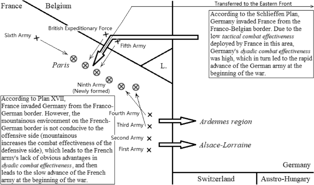
Schematic diagram of changes in the distribution of tactical combat effectiveness in France and Germany (August–September, 1914). Note:” × ” indicates the tactical combat effectiveness distribution of France in August, and “” indicates the distribution in September. ”→ ” indicates the trajectory of the position change

The preceding example illustrates how incorrect military deployment (non-subjective intention) can affect the variability of tactical combat effectiveness. There are also instances where commanders intentionally manipulate this variability—one such tactic is known as the “Defensive Feint Trap.” This strategy involves luring the enemy into a trap by feigning weakness, as depicted in Fig. 3. The essence of this tactic is to induce the opponent to misjudge the combat conditions, mistakenly believing they hold an advantage in tactical combat effectiveness by concealing their own operational capabilities. When the opponent launches an attack, they can be drawn into a precarious position where their tactical combat effectiveness is dramatically disadvantaged. The “defensive feint” tactic is somewhat akin to incorrect military deployment, differing only in whether the action is intentional.

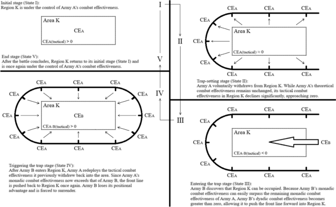
Schematic diagram of the “defensive feint trap” and its essence

On September 4, 1914, Graf Helmut von Moltke (Moltke the Younger), the chief of the German General Staff, was alarmed by the German army’s failure to capture many prisoners and military equipment during their advance. He mistakenly believed the French were retreating to lure the Germans deeper into their territory (Terraine 1960). In reality, this situation arose from the scarcity of equipment and personnel initially deployed by the French, resulting in low tactical combat effectiveness on the Franco-Belgian border. Thus, the distinction lies solely in whether the French deliberately chose not to utilize their combat effectiveness in the direction of Belgium during the early stages of the war.

Another tactic that leverages the dynamism of tactical combat effectiveness is the “principle of concentration of forces.” This tactic essentially involves concentrating combat power in a specific area when theoretical combat effectiveness is inferior to that of the opponent, relying on superior tactical combat effectiveness in that region to achieve localized victories.

Example IV

Ancient nomadic peoples typically possessed a lower theoretical combat effectiveness compared to organized states reliant on agricultural production and trade, but they could concentrate their tactical combat effectiveness in remote areas for looting. While such actions would likely provoke fierce reprisals from the imperial army, as long as they evacuated before the empire could activate its higher tactical combat effectiveness, they could remain safe.

In addition, the dynamics of tactical combat effectiveness are also influenced by non-military factors.

Example V

During the Afghan Civil War in the summer of 2021, the frontline advanced rapidly toward the Afghan government forces, indicating that CE_{Taliban-Afghan government forces} > 0. However, in August, the Taliban abruptly halted their advance when the front line reached the outskirts of Kabul, which means CE_{Taliban-Afghan government forces} = 0. These two situations are not contradictory. While the gap in theoretical combat effectiveness between the Taliban and Afghan government forces may not significantly narrow in the short term, their tactical combat effectiveness can change when the Taliban decides to suspend its use of combat effectiveness. Given that Afghanistan had been devastated by war since 1979, the destruction of Kabul would be extremely unfavorable for the incoming Taliban regime. Therefore, they became more inclined to prioritize peace talks to achieve their objectives.

Example VI

Similarly, in the Chinese Civil War after 1947, the People’s Liberation Army (PLA) rapidly advanced the frontline toward the National Revolutionary Army (NRA), indicating that CE_PLA-NRA > 0. However, in 1949, while advancing toward the cultural center of Beijing and the economic center of Shanghai, the front line temporarily halted (CE_PLA-NRA = 0). This was due to the significant damage inflicted on China’s economy and culture during the Japanese invasion from 1931 to 1945. It was more advantageous for the newly emerging state to incorporate Beijing and Shanghai into their sphere of power control through peace talks than to occupy them destructively using combat effectiveness. Consequently, the PLA temporarily reduced its tactical combat effectiveness to zero by halting its military actions. Fu Zuoyi, the supreme military officer of the NRA in the Beijing area, agreed to the peace proposal. In contrast, Tang Enbo, the supreme military officer of the NRA in the Shanghai area, rejected the offer. As a result, the PLA resumed its tactical combat effectiveness, and as CE_PLA-NRA became greater than zero again, the front line advanced into Shanghai.

Now, let us summarize the previously discussed scenarios, highlighting instances where tactical combat effectiveness diverges from theoretical combat effectiveness through a comprehensive example.

Example VII

In the ongoing Russo-Ukrainian War, during the early stages, following the failure of Russia’s surprise attack tactics and the rapid and substantial aid provided by NATO to Ukraine, Russia came to realize that its strategic plan to conquer the entirety of Ukraine was no longer achievable. Consequently, they decided to withdraw from Kyiv at the end of March 2022. This decision is similar to the previously mentioned tactic of nomadic tribes, which involved concentrating combat effectiveness in a specific area. While Russia’s theoretical combat effectiveness would not significantly change in the short term, the tactic resulted in an initial decrease (due to the withdrawal of combat effectiveness from western Ukraine) followed by an increase (as combat effectiveness was reallocated to eastern Ukraine) in the tactical combat effectiveness on the Ukrainian battlefield. Figure 4 illustrates the daily values of Russia’s dyadic tactical combat effectiveness against Ukraine, measured in units of 24 h. The graph clearly shows the emergence of the A-wave trough at the end of March 2022. The decline to the left of this trough reflects the short-term drop in Russia’s tactical combat effectiveness resulting from the withdrawal from Kyiv. However, once this portion of combat effectiveness was redirected via Belarus to eastern Ukraine, the tactic of concentrating combat effectiveness began to take effect, as indicated by the rise to the right of the A trough.

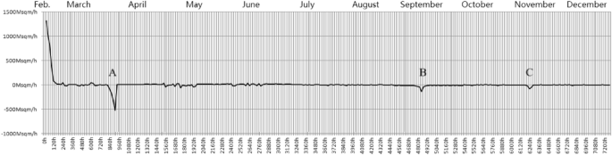
Daily Russian Tactical Combat Effectiveness Relative to Ukraine in 2022. Note: Data on daily Two-Dimensional Frontline Advancement Rate in Russia is sourced from respected military analysis platforms such as the Institute for the Study of War (ISW, https://www.understandingwar.org/) and Political Geography Now (PolGeoNow, https://www.polgeonow.com/). These datasets are derived from traditional frontline reporting, high-resolution satellite imagery, and shortwave infrared monitoring of fire points. Prominent military commentators, including Poulet Volant (https://twitter.com/Pouletvolant3) and War Mapper (https://twitter.com/war_mapper), have also analyzed the scale of frontline changes on the Russo-Ukrainian battlefield, publishing their calculations on Twitter. Their contributions serve as valuable cross-references, enhancing the reliability and accuracy of our data

In September 2022, Ukraine regained control of the Kharkiv region. This was due not only to the return of NATO-trained Ukrainian reservists to the battlefield, but also to Ukraine’s use of feint tactics. They created the illusion of an offensive toward Zaporizhzhia and Kherson, leading Russia to deploy a significant amount of tactical combat effectiveness in defense in the southeastern region of Ukraine. Consequently, despite Russia’s overall theoretical combat effectiveness remaining unchanged, its tactical combat effectiveness in northeastern Ukraine became relatively weak, similar to the situation of France before the First Battle of the Marne. The decline to the left of the B trough (the decrease in Russia’s dyadic combat effectiveness against Ukraine) captures this dynamic.

The rise to the right of the B trough (reflecting an increase in Russia’s dyadic combat effectiveness) occurred due to Ukraine temporarily halting its tactical combat effectiveness. After recapturing the Kharkiv region, Ukrainian forces advanced to the Russia-Ukraine border. However, they voluntarily halted their advance at the brink of entering Russian territory, influenced by NATO’s reluctance to support an offensive into Russian territory and Russia’s nuclear warnings concerning homeland security at that time. This decision parallels the Taliban’s restraint in advancing into Kabul and the PLA’s pause in exercising tactical combat effectiveness upon reaching Beijing. Ukraine’s decision to halt its advance led to a decrease in its tactical combat effectiveness, thereby allowing Russia’s dyadic combat effectiveness to rise once again.

By November 2022, Ukraine regained control of the western part of Kherson Province, including the capital city of Kherson, which is reflected in the decline to the left of the C trough. The rise to the right of the C trough similarly occurred due to Ukraine pausing its tactical combat effectiveness after securing victory. This time, the interfering factor was the Dnieper River. As the fourth-largest river in Europe, its wide expanse made it even more difficult for Ukraine to rapidly deploy tactical combat effectiveness from the western bank to the eastern bank. Moreover, the risk of a man-made dam breach at the Dnipro River dam, located in the upstream Russian-occupied area, further exacerbated the challenges of deploying tactical combat effectiveness across the river.

The distinction between tactical combat effectiveness and theoretical combat effectiveness also addresses the questions raised in earlier chapters: why do countries with significant disparities in comprehensive national power exhibit seemingly equal combat effectiveness during the Korean War and the Russo-Ukrainian War? The answer lies in the fact that it is the tactical combat effectiveness that is equal, not the theoretical combat effectiveness. This situation can be likened to a tug-of-war competition between an adult and a child. While it is widely recognized that the adult possesses superior physical strength, if the adult is unable to fully exert their strength for various reasons, and the child employs tools to enhance their power, thereby exceeding their natural abilities, it is not surprising that both sides reach a stalemate where the rope remains stationary. Specifically:

Explanation of the causes for “CE = 0” in example II

During the Korean War, the tactical combat effectiveness of the United States was significantly lower than its theoretical combat effectiveness. On one hand, by 1950, five years after the end of World War II, many World War II veterans had retired from the military and were reluctant to return to combat. On the other hand, the mountainous terrain greatly restricted the mobility of U.S. mechanized forces, preventing the U.S. military’s greatest advantage—advanced technological equipment—from functioning effectively. In contrast, the tactical combat effectiveness of the Chinese military exceeded its theoretical combat effectiveness. This was partly because the terrain was more conducive to the Chinese military’s typical tactics (e.g., night operations, surprise attacks, ambushes), leading to increased tactical combat effectiveness on their side. Additionally, the Soviet Union enhanced its military assistance to China during the war and even deployed some air force units (Wang 2000, 150–151). These factors ultimately resulted in a situation in the early 1950s where, despite a significant disparity in theoretical combat effectiveness between the two countries, their tactical combat effectiveness on the Korean battlefield was roughly equal.

Explanation of the causes for “CE = 0” in example III

The tactical combat effectiveness that Russia employed on the Ukrainian battlefield was lower than its theoretical combat effectiveness. This was due to a limited mobilization; the invasion of Ukraine resulted in significant international moral condemnation and strict economic sanctions, making the costs of expanding and escalating the war prohibitively high. In contrast, Ukraine’s tactical combat effectiveness was higher than its theoretical combat effectiveness. On one hand, Ukraine engaged in a nationwide mobilization under the rallying cry of defending the homeland. On the other hand, substantial support from NATO enabled Ukraine to demonstrate combat effectiveness that surpassed its theoretical limits. As these factors gradually formed a negative feedback balance, it became increasingly difficult for either side to effect significant changes in the front lines. This dual feedback loop can be macroscopically described as:

1. Russia adjusts tactics or strengthens mobilization → 2. CE_{Russia-Ukraine} is higher than zero → 3. Russia advances the frontline → 4. The international community offers more assistance → 5. CE_{Russia-Ukraine} drops below zero → 6. Ukraine advances the frontline → 7. Russia is deploying more war resources, including increased personnel mobilization and military spending → 8. CE_{Russia-Ukraine} is higher than zero → and the cycle repeats and continues from stage 3.

To provide readers with a more intuitive understanding of this dual feedback loop, we have created Fig.5.

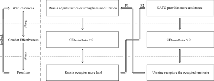
The Hyper-Stable Dual Feedback Loop in the Russo-Ukrainian War. Notes: 1.From left to right: schematic diagram and live diagram. 2.From top to bottom: changes in “War Resources”, “Combat Effectiveness” and “Frontline” levels

The diagram illustrates that the cycle consists of two interlocking sets of “war resources—combat effectiveness—frontline” feedback mechanisms, forming a closed-loop system where any change in the frontline will soon cause a change in the opposite direction. Therefore, despite the significant disparity in theoretical combat effectiveness between Russia and Ukraine, the tactical combat effectiveness demonstrated on the Ukrainian battlefield remains roughly equal. The stalemate will only be broken under one of two scenarios: (1) Russia reaches the mobilization limit of its war resources, causing a breakdown in Feedback Loop 1 (F1), or (2) “Ukraine fatigue” leads NATO to suspend its assistance, resulting in a breakdown in Feedback Loop 2 (F2). Ultimately, the outcome of the Russo-Ukrainian War hinges on which of these scenarios materializes first.

Overall CE and staged CE

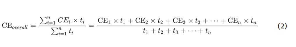
Overall combat effectiveness measures the average combat effectiveness over the entire course of a war, whereas staged combat effectiveness refers to combat effectiveness at a particular stage of the war. Since overall combat effectiveness is essentially a weighted average [3] of the combat effectiveness at various stages, the conversion formula between the two is:

Example VIII

During the initial eight years from the outbreak of the war to the signing of the Pacification of Ghent, the provinces of the Low Countries were united in their efforts, with their tactical combat effectiveness surpassing that of the Spanish garrisons in the region. Compared to the frontline in 1568, the frontline in 1576 encompassed an additional 72,000 square kilometers (Hooker 1999, p. 87). Based on this, it can be inferred that:

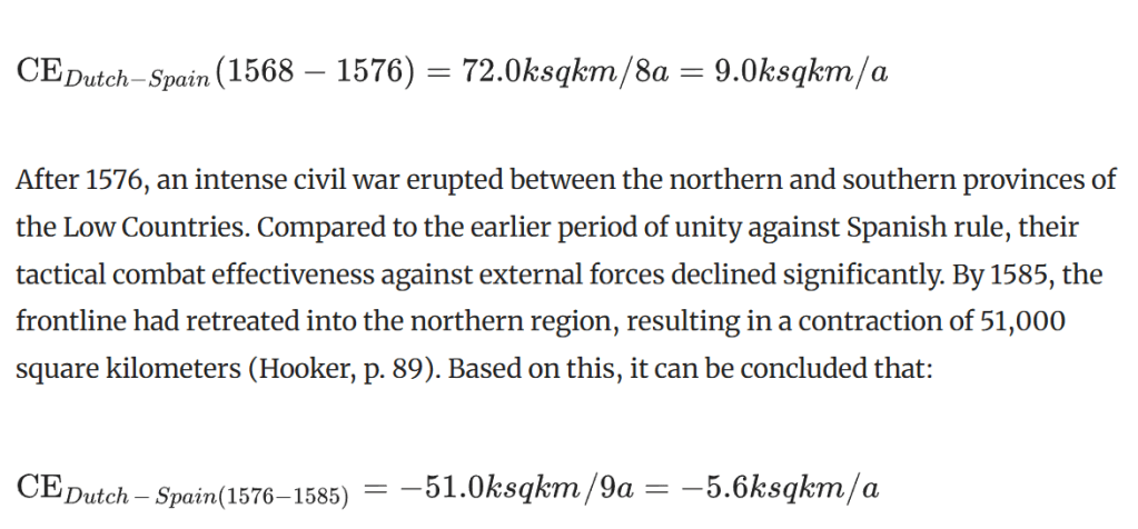
In 1588, the defeat of the Spanish Armada in its campaign against England significantly reduced the theoretical combat effectiveness of the Spanish Empire. Furthermore, the outbreak of war between the Spanish Netherlands and France in 1590 directly diminished Spain’s tactical combat effectiveness in the Netherlands, thereby increasing the dyadic combat effectiveness of the Dutch Republic. By the end of the war in 1648, the frontline had advanced southward to “more or less the present-day frontiers of Holland,” representing an expansion of 19,000 square kilometers (Hooker, p. 90). Based on this, it can be concluded that:

Using the above data, we can apply two methods to calculate the overall combat effectiveness of the Dutch side throughout the War of Independence.

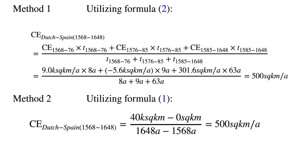
Clearly, using the measurement formula (Formula 1) directly is more straightforward than using the overall-stage combat effectiveness conversion formula (Formula (2)). Therefore, the conversion formula is not intended for calculating overall combat effectiveness; rather, it is more often used when the overall combat effectiveness and most stage combat effectiveness values are known, to determine an unknown stage combat effectiveness.

Example III

If we consider the broad starting point of the Russo-Ukrainian War—the time when Russian troops were sent to the Crimea Peninsula on February 24, 2014—over the past ten years, Russia has incorporated 108,900 square kilometers of Ukrainian land into its sphere of power control. So, according to Formula (1):

If we consider the narrow starting point of the Russo-Ukrainian War—starting from the time when Russia officially entered the conflict on February 24, 2022—over the past two years, Russia has incorporated 65,700 square kilometers of Ukrainian land into its sphere of power control. So, according to Formula (1):

By comparing these two values, we can observe that CE_overall is significantly lower than CE_{stage II}, amounting to only one-third of the latter. This is because during the 2014–22 period, Russia could not publicly convert its theoretical combat effectiveness into tactical combat effectiveness for direct deployment to the Ukrainian battlefield; instead, it could only support the pro-Russian separatist forces in eastern Ukraine against the Ukrainian government troops through covert means of supplying war resources. This clearly dragged down the overall combat effectiveness on the Russian side. With the known overall combat effectiveness of Russia from 2014 to 2022 and the stage II combat effectiveness from 2022 to 2024, we can easily determine the combat effectiveness during the phase when Russia did not directly participate in the war (let CE_{Russia—Ukraine (Feb. 2014–Feb. 2022)} = CE_{stage I} = x) using the conversion formula. The calculation method is based on Formula (2):

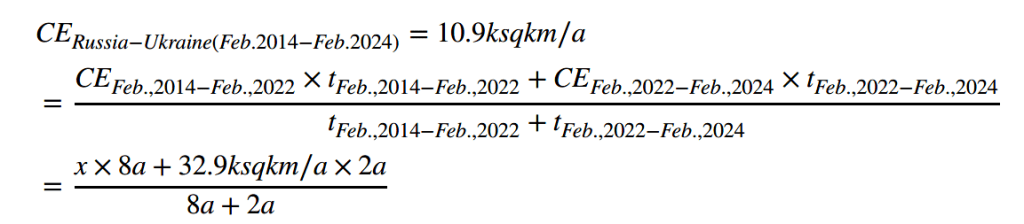
Solving the equation gives us x = 5.4 ksqkm/a.

CE_{stage I} is less than one-sixth of CE_{stage II} and less than half of CE_overall. This quantifies the extent to which the combat effectiveness of the Russian side has been dragged down by the pro-Russian separatists in eastern Ukraine, relying solely on Russian military resources and technical support.

Conclusion

This paper presents a concise, universally applicable, and objective method for measuring dyadic tactical combat effectiveness—namely, the Two-Dimensional Frontline Advancement Rate (TFR) method. Its conciseness stems from the fact that it requires only two easily obtainable parameters: the spatial extent of frontline advancement and the temporal span. The universality of this method is demonstrated by its applicability to all forms of power struggles, even including urban gang confrontations and territorial disputes among animals, as long as clear boundaries of power are established. Its objectivity is grounded in the fact that these parameters are objective physical quantities, independent of human subjective perception.

Consequently, the most significant contribution of this paper lies in the quantification of the most direct outcomes of war—victory, draw, and defeat (categorical variables)—through the utilization of changes in the front line (a quantitative variable). This is analogous to the way natural sciences use temperature (a quantitative variable) to quantify cold, moderate, and hot (categorical variables), or employ speed (a quantitative variable) to quantify fast, medium, and slow (categorical variables). In fact, the very approach of using quantitative variables to tautologically describe unquantifiable categorical variables is the core idea of measurement science.

More specifically, our contribution lies in the discovery of a method to quantify changes in the front line by calculating the area enclosed between the new front line formed after the change and the original front line prior to the change, measured per unit of time. This addresses a long-standing challenge faced by researchers: the inability to accurately quantify changes in the front line using only the one-dimensional frontline advancement rate, which in turn hindered the precise quantification of victory, stalemate, and defeat (Fig. 6).

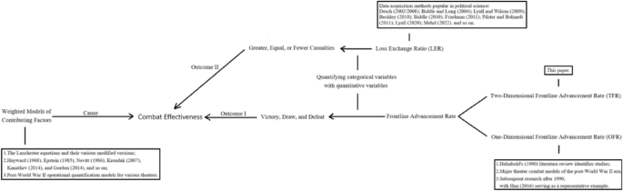
The academic development map of combat effectiveness measurement problems and the position of this paper (its contribution to the field)

Furthermore, the contribution of this paper includes a clear delineation of three sets of classifications for combat effectiveness: “monadic vs. dyadic,” “theoretical vs. tactical,” and “overall vs. staged,” along with seven illustrative examples. These examples encompass various types of wars throughout history, including guerrilla warfare by nomadic tribes against agrarian empires (Example IV, Ancient), the Eighty Years’ War (Example VII, 1568-1648), World War I (Example I, 1914-1918), the Chinese Civil War (Example VI, 1946-1949), and the Korean War (Example II, 1950-1953). Additionally, it includes the recently concluded Afghan Civil War (Example V, 2021) and the ongoing Russo-Ukrainian War (Example III, from 2014/2022 to the present).

By classifying and defining combat effectiveness, we clarify the applicable types of the TFR method. This method differs from previous operations research approaches that aim to predict and assess “monadic” and “theoretical” combat effectiveness based on explanatory variables. Since monadic combat effectiveness is not necessarily correlated with battle outcomes—results also depend on whether the opponent is relatively stronger—and theoretical combat effectiveness is similarly not necessarily correlated with battle outcomes, as the results depend on the efficiency of its conversion on the battlefield, a particularly noteworthy distinction emerges: when using explanatory variables to measure combat effectiveness, one should not aim for consistency between combat effectiveness and combat outcomes. Talmadge (2013), Castillo (2014) and Brathwaite (2018) have conducted meaningful discussions on this issue.

In contrast, the TFR method aligns more closely with the LER method commonly used in political science, as both are outcome-based and aim to measure dyadic tactical combat effectiveness. Both methods take into account the combat effectiveness of opponents [4] and are influenced by the actual combat environment on the battlefield. The relationship between LER and TFR is like that of different thermometers (mercury thermometers and infrared forehead thermometers) made respectively by utilizing different outcomes of temperature (changes in metal volume and infrared radiation intensity)—they share the same measurement concept, but each has its own unique advantages.

It is evident that discussing the application conditions of the method for measuring combat effectiveness should not only focus on the types of wars to which it is applicable but also consider the types of combat effectiveness it is designed to measure. Summarizing the preceding discussions, we can conclude that in terms of applicable war types, the TFR method is suitable for all wars involving frontlines, not merely those aimed at territorial acquisition. Similarly, the LER method applies to all wars involving soldier casualties, not just those motivated by revenge or killing. Regarding the types of combat effectiveness, both the TFR and LER methods are specifically designed to measure dyadic tactical combat effectiveness.

It is precisely because of these significant similarities with the LER method that the TFR method can also serve as a viable approach for acquiring data in the most common statistical modeling research in the current field of political science. For instance, we utilized the TFR method to obtain daily measurements of Russia’s dyadic tactical combat effectiveness relative to Ukraine since February 24, 2022. Using this time series data, comprising nearly 1,000 samples, we established an ECM model to evaluate the impact of international prices for oil, iron ore, and wheat on Russia’s combat effectiveness. Furthermore, we developed a GARCH model to analyze the volatility trends of Russia’s dyadic tactical combat effectiveness. Additionally, leveraging the daily reports published by the Ukrainian General Staff, we constructed VAR and ARIMA models to investigate the functional relationship between Russia’s war losses and its territorial expansion. We also observed that rapid changes in the front line are often more evident during naval and aerial battles. This is because, compared to ground combat, naval and aerial warfare rely more heavily on advanced weaponry and cutting-edge military technology, resulting in more pronounced disparities in combat effectiveness.

Currently, the primary challenge facing the TFR method is the lack of a comprehensive database. For example, the studies mentioned above are limited to the Russo-Ukrainian War because it is the first conflict in world history to be continuously reported on by the media, enabling the collection of daily time-series data on frontline changes. Previous conflicts lack such detailed resources. Unlike the LER method, which can draw on datasets of combat losses for nearly all wars since 1492 (see Clodfelter 2017), and other databases such as COW, CDB-90, and Jason Lyall’s Project Mars, the data required for the TFR method currently must be extracted from historical maps and calculated using area measurement software. Therefore, we have a follow-up plan to measure the frontline changes in historical wars throughout human history. This effort could potentially lead to the establishment of a database of combat effectiveness measured using the TFR method, which would serve as a valuable resource for researchers to construct military mathematical models and develop military simulation software.

Notes:

1. Finland’s casualty data are sourced from Kurenmaa and Lentilä (2005). For the Soviet Union, we currently have four different estimates, sourced from Krivosheyev (1997), Sokolov (2000), Kilin (2007), and Petrov (2013). We adopt the lowest estimate for Soviet losses. If the highest Soviet casualty estimate is used, Finland’s Loss Exchange Ratio (LER) rises to 6.485, while the Soviet Union’s LER drops to 0.154. Therefore, the LER data from the Winter War not only highlights the inconsistency between LER and the outcomes of victory, draw, or defeat but also underscores the first limitation discussed earlier: the LER method is highly susceptible to subjective factors in data collection and interpretation, leading to significant discrepancies.
2. In this context, the letter “T” is an SI prefix (International System of Units) denoting 10¹². The subsequent notations G(10⁹), M(10⁶), and k(10³)are also SI prefixes.
3. The weighted arithmetic mean is similar to an ordinary arithmetic mean, with the exception that some data points contribute more than others to the final average. For example, if the output value of an area is $1,000 in the first eight years of a ten-year period, and $2,000 in the next two years, then the average output value of that area across ten years is not (1000 + 2000)/2 = $1500, but (1000 × 8 + 2000 × 2)/10 = $1200. Or, to continue with the car speed example, if the speed of a car is 100km/h for the first 2 h, 80km/h for the next 3 h, and 60km/h for the last 5 h, then the overall speed of the car is not (100 + 80 + 60)/3 = 80km/h, but (100 × 2 + 80 × 3 + 50 × 5)/10≈69km/h.
4. Interestingly, the combat effectiveness values of the two warring parties derived from the TFR method are always additive inverses (CE_A-B + CE_B-A = 0), as changes in the area caused by frontline shifts adhere to the principles of a zero-sum game. In contrast, the combat effectiveness values of the two warring parties derived from the LER method are always reciprocals (CE_A/B × CE_B/A = 1), as one side’s inflicted casualties are precisely the other side’s combat losses. These straightforward mathematical relationships reflect the fundamental nature of both methods: they measure dyadic combat effectiveness by fully accounting for the opponent’s combat effectiveness.

References:

Apostolou, C. 2015. The dictator’s army: Battlefield effectiveness in authoritarian regimes. Cornell University Press.

Banks, A. 1989. A military atlas of the first world war. Pen & Sword Books Ltd.

Beckley, M. 2010. Economic development and military effectiveness. The Journal of Strategic Studies 33 (1): 43–79.

Biddle, S. 2006. Military power: Explaining victory and defeat in modern battle. Princeton University Press.

Biddle, S. 2010. Military effectiveness. In The international studies encyclopedia, ed. R.A. Denemark, xx–xx. Wiley-Blackwell.

Biddle, S., and S. Long. 2004. Democracy and military effectiveness: A deeper look. Journal of Conflict Resolution 48 (4): 525–546.

Brathwaite, K.J.H. 2018. Effective in battle: Conceptualizing soldiers’ combat effectiveness. Defence Studies 18 (1): 1–24.

Brooks, R., and E.A. Stanley. 2007. Creating military power: The sources of military effectiveness. Stanford University Press.

Castillo, J. 2014. Endurance and war: The national sources of military cohesion. Stanford: Stanford University Press.

Clodfelter, M. (2017). Warfare and armed conflicts: A statistical encyclopedia of casualty and other figures, 1492–2015 (4th ed.). McFarland.

Desch, Michael C. 2002. Democracy and victory: Why regime type hardly matters. International Security 27 (2): 5–47.

Desch, M.C. 2008. Power and military effectiveness: The fallacy of democratic triumphalism. Johns Hopkins University Press.

Dolanský, L. 1964. Present state of the Lanchester theory of combat. Operations Research 12 (2): 344–358.

Downes, A.B. 2009. How smart and tough are democracies? Reassessing theories of democratic victory in war. International Security 33 (4): 9–51.

Dupuy, T.N. 1987. Understanding war: History and theory of combat. Leo Cooper.

Epstein, J. 1985. The calculus of conventional war: Dynamic analysis without Lanchester theory. Brookings Institution Press.

Farrell, T. 2005. World culture and military power. Security Studies 14 (3): 448–488.

Friedman, J.A. 2011. Manpower and counterinsurgency: Empirical foundations for theory and doctrine. Security Studies 20 (4): 556–591.

Gordon, D. 2014. Electronic warfare: Element of strategy and multiplier of combat power. Pergamon Press.

Grauer, R. 2016. Commanding military power: Organizing for victory and defeat on the battlefield. Cambridge University Press.

Grauer, R., and S.L. Quackenbush. 2021. Initiative and military effectiveness: Evidence from the Yom Kippur War. Journal of Global Security Studies 6 (2): 191–205.

Halberstam, D. 2007. The coldest winter: America and the Korean War. Hyperion Publishing.

Han, S.J. 2016. Analysis of relative combat power with expert system. Journal of Digital Convergence 14 (6): 143–150.

Hayward, P. 1968. The measurement of combat effectiveness. Operations Research 16 (2): 314–323.

Helmbold, R. 1990. Rates of advance in historical land combat operations (CAA-RP-90–1). Bethesda: US Army Concepts Analysis Agency.

Helmbold, R. (1997). The advantage parameter: A compilation of Phalanx articles dealing with the motivation and empirical data. Army Concepts Analysis Agency.

Hooker, M. 1999. The history of Holland. Greenwood Publishing Group.

Johnson, P.B. 2012. Does decapitation work? Assessing the effectiveness of leadership targeting in counterinsurgency campaigns. International Security 36 (4): 47–79.

Kanatliev, R. (2014). Improving relative combat power estimation: The road to victory. Army Command and General Staff College.

Kier, E. 1998. Homosexuals in the US military: Open integration and combat effectiveness. International Security 23 (2): 5–39.

Kilin, J. (2007). Rajakahakan hidas jäiden lähtö. In M. Jokisipilä (Ed.), Sodan totuudet: Yksi suomalainen vastaa 5.7 ryssää [Truths of War: One Finn equals 5.7 Russians]. Helsinki, Finland: Ajatus Kirjat. [Author’s translation]

Krivosheyev, G.F. 1997. Soviet casualties and combat losses in the twentieth century, 1st ed. London, UK: Greenhill Books.

Krondak, W. J., Cunningham, R., Hunsaker, O., Derendinger, D., Cunningham, S., & Peck, M. (2007). Unit combat power (and beyond). Paper presented at the 24th international symposium on military operational research (ISMOR), August 28–31, 2007.

Kuo, K. 2022. Dangerous changes: When military innovation harms combat effectiveness. International Security 47 (2): 48–87.

Kurenmaa, P., & Lentilä, R. (2005). Sodan tappiot [Casualties of the War]. In J. Leskinen & A. Juutilainen (Eds.), Jatkosodan pikkujättiläinen (in Finnish). Helsinki, Finland: Werner Söderström Osakeyhtiö.

Lanchester, F. (1916). Aircraft in warfare: The dawn of the fourth arm. Constable Ltd.

Levine, P. 2013. The British empire: Sunrise to sunset. Pearson Education Limited.

Lyall, J. 2020. Divided armies: Inequality and battlefield performance in modern war. Princeton University Press.

Lyall, J., and I.I.I.I. Wilson. 2009. Rage against the machines: Explaining outcomes in counterinsurgency wars. International Organization 63 (1): 67–106.

McKenna. A.. Britannica Online, s.v. “combat-effectiveness”, URL =<https://www.britannica.com/topic/combat-effectiveness>.

Mehrl, M. 2022. Female combatants and rebel group behaviour: Evidence from Nepal. Conflict Management and Peace Science 40 (3): 260.

Millett, A.R., W. Murray, and K.H. Watman. 1986. The effectiveness of military organizations. International Security 11 (1): 37–71.

Millett, A. R., & Murray, W. (Eds.). (2010). Military effectiveness (Vols. 1–3). Cambridge University Press.

Novikov, D.A. 2013. Hierarchical models of warfare. Automation and Remote Control 74 (10): 1733–1752.

Obermeyer, Z., C.J. Murray, and E. Gakidou. 2008. Fifty years of violent war deaths from Vietnam to Bosnia: Analysis of data from the world health survey programme. BMJ 336 (7659): 1482–1486. https://doi.org/10.1136/bmj.a137.

Perry, N. (2009). Fractal effects in Lanchester models of combat. Australian joint operations division defense science and technology organization report. URL = https://www.onacademic.com/detail/journal_1000032543464210_151e.html.

Petrov, P. (2013). Venäläinen talvisotakirjallisuus: Bibliografia 1939–1945 [Russian Winter War Literature: Bibliography 1939–1945] (in Finnish). Jyväskylä, Finland: Docendo.

Pilster, Ulrich, and Tobias Bohmelt. 2011. Coup-proofing and military effectiveness in interstate wars, 1967–99. Conflict Management and Peace Science 28 (4): 331–350.

Plapinger, S.H. 2022. Insurgent recruitment practices and combat effectiveness in civil war: The black September conflict in Jordan. Security Studies 31 (2): 251–290.

Pollack, K.M. 2002. Arabs at war: Military effectiveness. University of Nebraska Press.

Przemieniecki, J.S. 2000. Mathematical methods in defense analyses. The American Institute of Aeronautics and Astronautics.

Reiter, D., ed. 2017. The sword’s other edge: Trade-offs in the pursuit of military effectiveness. Cambridge University Press.

Reiter, D. 2020. Avoiding the coup-proofing dilemma: Consolidating political control while maximizing military power. Foreign Policy Analysis 16 (3): 312–331.

Reiter, D. 2022. Command and military effectiveness in rebel and hybrid battlefield coalitions. Journal of Strategic Studies 45 (2): 211–233.

Reiter, D., and A.C. Stam III. 1998. Democracy and battlefield military effectiveness. Journal of Conflict Resolution 42 (3): 259–277.

Sokolov, B. (2000). Пyть к миpy [Secrets of the Russo-Finnish War]. Moscow, Russia: Veche.

Talmadge, C. 2013. The puzzle of personalist performance: Iraqi battlefield effectiveness in the Iran-Iraq war. Security Studies 22 (2): 180–221.

Terraine, J. 1960. Mons, the retreat to victory. Wordsworth Military Library.

Tolk, A. 2012. Engineering principles of combat modeling and distributed simulation. Wiley.

von Clausewitz, C. 1976. On war. Princeton: Princeton University Press.

Wang, H. 2000. My combat career. Central Party Literature Publisher.

Autore: Weipu Sun and Jiesheng Wang Joint

Fonte: International Politics February 2025